Introduction to locally weighted linear regression (Loess)

What is Locally Weighted Linear Regression?

Locally weighted linear regression is a non-parametric algorithm, combines different types of regression models in a k-nearest-neighbor model. Locally weighted regression is called LOESS. LOESS combines much of the simplicity of linear least squares regression with the flexibility of nonlinear regression.

Locally Weighted regression is memory-based work that performs regression at a point using the training data that are local to a point. In Loess for each linear model we would like to suit, we discover some extent x and use that for fitting a local regression model.

The estimator variance is minimized when the general includes as many training points as can be accommodated by the model. Too large a general includes points that degrade the fit, too small a general neglect points that increase confidence in the fit

Local regression illustrated on some simulated data, Here simple regression curve is represented by orange and the Locally weighted regression curve is represented by green.

Suppose If we want to evaluate the hypothesis of h at a certain local point x. For linear regression we do the following procedure:
Fit $θ$ to minimize $\sum_{i = 1}^{m} (y^{(i)} - θ^{T} x^{(i)})^{2}$
Output $θ^{T} x$
For locally weighted linear regression we will instead do the following:
Fit $θ$ to minimize $\sum_{i = 1}^{m} w^{(i)} (^{(i)} y - θ^{T} x^{(i)})^{2}$
Output $θ^{T} x$
A fairly standard choice for the weights is the following bell-shaped function:
$w^{(i)} = \exp (- \frac{(x^{(i)} - x)^{2}}{2 τ^{2}})$
Note that this is just a bell-shaped curve, not a Gaussian probability function.
Here the weights depend upon the certain local point x at which we are evaluating linear regression The parameter $τ$ controls how quickly the weight of a training example falls off with its distance the query point $x$ and is called the \textbf{bandwidth} parameter. In this case, increasing

$τ$ $τ$
$τ$ $τ$ increases the "width" of the bell shape curve and makes further points have more weight.

$τ$ $τ$ It $x$ is a vector, then this generalizes to be:
$w (i) = exp (- ( x ( i ) - x ) T ( x ( i ) - x ) 2 τ 2)$
$w (i) = exp (- ( x ( i ) - x ) 2 2 τ 2)$

The above figures are some of the examples of locally weighted linear regression with 3 and 5 data points.

The Relationship of Kernel Regression and Locally Weighted Regression

LWR has more advantages than Keneral Regression. For a Planar local model, LWR is far better than Keneral regression since LWR will exactly produce a straight line as compared to keneral regression.

LWR methods with a 4 quarter local model should fail to reproduce a cubic function, and so on.

Advantages

Loess did not require any specification of a function to fit into a model of sample data.

It is a supervised learning algorithm and extended form of linear regression

It is non-parametric, and no training phase exists in this only testing.

To avoid overfitting Loess allows us to put less care in selecting features in the data set.

Low dimension supervised learning.

Disadvantages

It requires a total training set to be to predict future predictions.

As the size of the training set increases linearly parameters also get increases.

Computationally intensive, as a regression model is computed for each point.

Like other least square methods, prone to the effect of outliers in the data set.

Deriving the vectorized implementation

Consider the 1D case where $Θ = [θ_{0}, θ_{1}]$ and $x$ and $y$ are vectors of size $m$ . The cost function $J (θ)$ is a weighted version of the OLS regression, where the weights $w$ are defined by some kernel function

\begin{aligned} J (θ) & = \sum_{i = 1}^{m} w^{(i)} {(y^{(i)} - (θ_{0} + θ_{1} x^{(i)}))}^{2} \\ \frac{\partial J}{\partial θ_{0}} & = - 2 \sum_{i = 1}^{m} w^{(i)} (y^{(i)} - (θ_{0} + θ_{1} x^{(i)})) \\ \frac{\partial J}{\partial θ_{1}} & = - 2 \sum_{i = 1}^{m} w^{(i)} (y^{(i)} - (θ_{0} + θ_{1} x^{(i)})) x^{(i)} \end{aligned}

Canceling the $- 2$ terms, equating to zero, expanding and rearranging the terms:

\begin{aligned} \frac{\partial J}{\partial θ_{0}} = \sum_{i = 1}^{m} w^{(i)} (y^{(i)} - (θ_{0} + θ_{1} x^{(i)})) = 0 \\ \sum_{i = 1}^{m} w^{(i)} θ_{0} + \sum_{i = 1}^{m} w^{(i)} θ_{1} x^{(i)} = \sum_{i = 1}^{m} w^{(i)} y^{(i)} & Eq. (1) \\ \frac{\partial J}{\partial θ_{1}} = \sum_{i = 1}^{m} w^{(i)} (y^{(i)} - (θ_{0} + θ_{1} x^{(i)})) x^{(i)} = 0 \\ \sum_{i = 1}^{m} w^{(i)} θ_{0} + \sum_{i = 1}^{m} w^{(i)} θ_{1} x^{(i)} x^{(i)} = \sum_{i = 1}^{m} w^{(i)} y^{(i)} x^{(i)} & Eq. (2) \end{aligned}

Writing Eq. (1) and Eq. (2) in matrix form $A Θ = b$ allows us to solve for $Θ$

$Θ$

\sum i = 1 m w (i) θ 0 + \sum i = 1 m w (i) θ 1 x (i) = \sum i = 1 m w (i) y (i) \sum i = 1 m w (i) θ 0 + \sum i = 1 m w (i) θ 1 x (i) x (i) = \sum i = 1 m w (i) y (i) x (i) [\sum w (i) \sum w (i) x (i) \sum w (i) x (i) \sum w (i) x (i) x (i)] [θ 0 θ 1] = [\sum w (i) y (i) \sum w (i) y (i) x (i)] A Θ = b Θ = A - 1 b

\sum i = 1 m w (i) θ 0 + \sum i = 1 m w (i) θ 1 x (i) = \sum i = 1 m w (i) y (i) \sum i = 1 m w (i) θ 0 + \sum i = 1 m w (i) θ 1 x (i) x (i) = \sum i = 1 m w (i) y (i) x (i) [\sum w (i) \sum w (i) x (i) \sum w (i) x (i) \sum w (i) x (i) x (i)] [θ 0 θ 1] = [\sum w (i) y (i) \sum w (i) y (i) x (i)] A Θ = b Θ = A - 1 b

CODE :

Implementation in python

import matplotlib.pyplot as plt
import pandas as pd
import numpy as np
from math import ceil
from scipy import linalg
from IPython.display import Image
from IPython.display import display
plt.style.use('seaborn-white')
%matplotlib inline

import numpy as np
from scipy import linalg

#Defining the bell shaped kernel function - used for plotting later on
def kernel_function(xi,x0,tau= .005): 
    return np.exp( - (xi - x0)**2/(2*tau)   )

def lowess_bell_shape_kern(x, y, tau = .005):
    """lowess_bell_shape_kern(x, y, tau = .005) -> yest
    Locally weighted regression: fits a nonparametric regression curve to a scatterplot.
    The arrays x and y contain an equal number of elements; each pair
    (x[i], y[i]) defines a data point in the scatterplot. The function returns
    the estimated (smooth) values of y.
    The kernel function is the bell shaped function with parameter tau. Larger tau will result in a
    smoother curve. 
    """
    m = len(x)
    yest = np.zeros(n)

    #Initializing all weights from the bell shape kernel function    
    w = np.array([np.exp(- (x - x[i])**2/(2*tau)) for i in range(m)])     
    
    #Looping through all x-points
    for i in range(n):
        weights = w[:, i]
        b = np.array([np.sum(weights * y), np.sum(weights * y * x)])
        A = np.array([[np.sum(weights), np.sum(weights * x)],
                    [np.sum(weights * x), np.sum(weights * x * x)]])
        theta = linalg.solve(A, b)
        yest[i] = theta[0] + theta[1] * x[i] 

    return yest

$Θ$

Implementation in Python using span kernel and robustyfing

iterations

from math import ceil
import numpy as np
from scipy import linalg

def lowess_ag(x, y, f=2. / 3., iter=3):
    """lowess(x, y, f=2./3., iter=3) -> yest
    Lowess smoother: Robust locally weighted regression.
    The lowess function fits a nonparametric regression curve to a scatterplot.
    The arrays x and y contain an equal number of elements; each pair
    (x[i], y[i]) defines a data point in the scatterplot. The function returns
    the estimated (smooth) values of y.
    The smoothing span is given by f. A larger value for f will result in a
    smoother curve. The number of robustifying iterations is given by iter. The
    function will run faster with a smaller number of iterations.
    """
    n = len(x)
    r = int(ceil(f * n))
    h = [np.sort(np.abs(x - x[i]))[r] for i in range(n)]
    w = np.clip(np.abs((x[:, None] - x[None, :]) / h), 0.0, 1.0)
    w = (1 - w ** 3) ** 3
    yest = np.zeros(n)
    delta = np.ones(n)
    for iteration in range(iter):
        for i in range(n):
            weights = delta * w[:, i]
            b = np.array([np.sum(weights * y), np.sum(weights * y * x)])
            A = np.array([[np.sum(weights), np.sum(weights * x)],
                          [np.sum(weights * x), np.sum(weights * x * x)]])
            beta = linalg.solve(A, b)
            yest[i] = beta[0] + beta[1] * x[i]

        residuals = y - yest
        s = np.median(np.abs(residuals))
        delta = np.clip(residuals / (6.0 * s), -1, 1)
        delta = (1 - delta ** 2) ** 2

    return yest

f = 0.25
yest = lowess_ag(x, y, f=f, iter=3)
yest_bell = lowess_bell_shape_kern(x,y)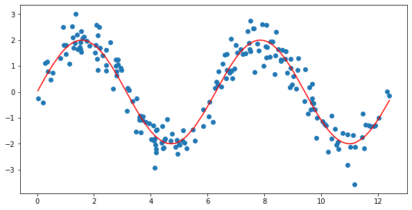

source: https://gist.github.com/agramfort/850437

REFERENCES:

https://www.olamilekanwahab.com/blog/2018/01/30/locally-weighted-regression/
https://gerardnico.com/data_mining/local_regression
https://www.ri.cmu.edu/pub_files/pub1/atkeson_c_g_1997_1/atkeson_c_g_1997_1.pdf

CONCLUSION:

By the Locally weighted regression, higher flexibility will obtained and desirable properties like smoothness and statistical analyzability will be retained.

Locally weighted learning is increasing rapidly in the machine learning community.

It minimizes the computational cost of training and new data points will store in the memory.

You must be clear while considering the learning algorithm since every algorithm has its own advantages.

Thanks for reading this.

\sum i = 1 m w (i) θ 0 + \sum i = 1 m w (i) θ 1 x (i) = \sum i = 1 m w (i) y (i) \sum i = 1 m w (i) θ 0 + \sum i = 1 m w (i) θ 1 x (i) x (i) = \sum i = 1 m w (i) y (i) x (i) [\sum w (i) \sum w (i) x (i) \sum w (i) x (i) \sum w (i) x (i) x (i)] [θ 0 θ 1] = [\sum w (i) y (i) \sum w (i) y (i) x (i)] A Θ = b Θ = A - 1 b

YELLANKI ABHINAV

Sunday, November 15, 2020

Locally Weighted Linear Regression (Loess)